
Valuation is a central component of many high-stakes commercial disputes, from shareholder appraisal actions and bankruptcy proceedings to tax controversies and breach-of-contract claims. In these contexts, the determination of a company’s fair market value often hinges on the present value of projected cash flows, making the discounting exercise a critical step in the valuation process.
In financial modeling, particularly when applying discounted cash flow (“DCF”) methods to estimate the value of a business or an asset, the discount rate plays a pivotal role in translating future cash flows into a present value.[1] Traditionally, practitioners apply a single discount rate to all future cash flows, reflecting the overall risk profile and the time value of money for the investment. In certain cases, however, the use of multiple discount rates may be considered more appropriate, particularly when future cash flows differ meaningfully in terms of risk, timing, or underlying economic conditions.
For instance, when a company or asset’s risk profile is expected to remain relatively stable over time, applying a single discount rate may provide a reasonable approximation of value. In contrast, when risks evolve materially across different phases of a business, such as in industries with distinct development and commercialization stages, a framework of multiple discount rates may better capture these changing risk characteristics.[2]
Because discounting compresses a range of future expectations into a single present value figure, even modest variations in the choice of methodology can lead to significant differences in the resulting valuation. The effect of discount rate selection on valuation can be particularly pronounced in litigation involving large, complex businesses, where valuations may reach into the billions of dollars.
Consequently, the choice between using a single discount rate or multiple rates is not merely a technical modeling decision; it can be a focal point of dispute, with significant legal and financial implications. Understanding the considerations that motivate each approach is therefore critical for litigators, experts, and courts as they assess the credibility and robustness of competing valuation analyses.
Discounted Cash Flow in Valuation Litigation
The DCF method is a commonly used tool in financial valuation and is frequently applied in both corporate finance and investment analysis. DCF estimates the present value of a business or asset by projecting its expected future cash flows and discounting those cash flows back to a selected point in time using an appropriate discount rate. The discount rate reflects the opportunity cost of capital (i.e., what investors could earn in an alternative investment of comparable risk) and incorporates both the time value of money and the uncertainty associated with receiving future cash flows.[3] It can be influenced by factors such as macroeconomic conditions, capital structure, and exposure to market risk.
The DCF model is widely accepted in enterprise valuation practice. It focuses on a business’s expected future performance, which is particularly important for companies with unique capital structures, limited public comparables, or evolving business models to consider. These company characteristics make DCF especially relevant in valuation-related litigation, where generating a case-specific, independent estimate of value is often paramount. For example, courts have relied on DCF in shareholder appraisal actions,[4] breach of fiduciary duty claims,[5] lost profits assessments,[6] and bankruptcy proceedings.[7]
DCF is among the valuation methods that have been considered by courts, including the Delaware Court of Chancery. For example, in In re Appraisal of Dell Inc., the Court emphasized that “the DCF . . . methodology has featured prominently in this Court because it is the approach that merits the greatest confidence within the financial community.”[8] Similarly, in Andaloro v. PFPC Worldwide, the Court stated that DCF “is frequently used in the Delaware Chancery Court and many prefer to give it great, and sometimes even exclusive, weight when it may be used responsibly.”[9]
A typical DCF analysis in enterprise valuation involves three key components: (1) projecting cash flows over a discrete forecast period, (2) estimating a terminal value to capture the value of cash flows beyond that horizon, and (3) applying a discount rate to convert future cash flows into present value. Each of these components can significantly affect the outcome and is often subject to dispute in litigation. Differences in projections, assumptions about terminal growth, or the construction of the discount rate can lead to materially different conclusions about value.
DCF valuations are sensitive to the selection of the discount rate and the methodology used to apply it. Because discounting compresses future cash flows into a single present value figure, small changes in the discount rate—or in the way rates are applied across time—can result in large changes in the final valuation. This sensitivity becomes especially consequential in high-stakes litigation, where valuations often involve complex, multi-billion-dollar businesses. The discussion that follows examines the considerations underlying the choice between a single and multiple discount rates approach, as well as the potential valuation consequences in litigation settings.
Single Discount Rate Approach
The single discount rate approach is the most common method in Discounted Cash Flow analysis. Under this approach, all projected future cash flows are discounted back to a particular time using a constant rate that reflects the overall risk profile of the business or asset. This rate captures both the time value of money and the risk associated with receiving those cash flows over time.
In practice, when valuing a firm’s free cash flows, the single discount rate is typically based on the firm’s weighted average cost of capital (“WACC”), which represents the average return required by all capital providers—both debt and equity. The capital asset pricing model (“CAPM”) is commonly used to price the required return to equity. CAPM calculates the cost of equity as the sum of the risk-free rate (the return on a virtually riskless investment, such as a U.S. Treasury bond), the market risk premium (the additional return expected from investing in the overall market above the risk-free rate), and the company’s beta (a measure of how sensitive the company’s equity returns are to movements in the overall market). A beta greater than one indicates higher systematic (undiversifiable) risk than the market, while a beta below one suggests lower market-related risk.
The cost of debt, by contrast, reflects the effective rate the firm pays on its borrowings, adjusted for the tax deductibility of interest. In practice, various approaches are used to estimate it, including using the firm’s current yield on debt or the sum of a risk-free rate and a credit spread that captures the firm’s default risk. The WACC combines these two components—the cost of equity and the after-tax cost of debt—weighted by their respective proportions in the firm’s capital structure.
Once determined, this single discount rate is applied to all projected cash flows, regardless of when they occur. This creates a consistent framework for evaluating a stream of future benefits based on a single measure of opportunity cost and risk exposure.[10]
To illustrate, consider a simplified model of a business that expects to generate $10 million in free cash flows annually for the next ten years, and assume the firm’s WACC is estimated at 12%.[11] The present value of this future cash flow stream is calculated as

This means the total present value of the ten-year $10 million annual cash flow stream, when discounted at a constant 12% rate, is approximately $56.5 million.
The single discount rate approach is often used in valuation models due to its conceptual clarity and ease of application, particularly when a firm’s risk profile and capital structure are expected to remain relatively stable over time. In cases where those factors vary meaningfully, however, applying a constant rate across all cash flows may not fully reflect the underlying economic characteristics of the business.
Multiple Discount Rates Approach
Traditional DCF models often apply a single discount rate to all projected cash flows, but a body of academic literature has raised concerns about the limitations of this assumption. Researchers have pointed to various settings where a constant discount rate may not reflect the economic characteristics of the underlying investment.[12]
First, several studies suggest that the required rate of return used in valuation models can vary over time due to changing economic conditions and the evolving opportunity cost of capital—that is, the return investors forgo by allocating funds to a specific project rather than to alternative investments. In such cases, the assumption of a constant discount rate may lead to valuation results that do not fully capture the time-varying risk profile of the investment.[13]
Second, some researchers argue that many investment projects exhibit nonconstant risk exposure over their life cycle, with distinct phases that carry different types and magnitudes of risk. For instance, a project may begin with high levels of idiosyncratic or technical uncertainty and later transition into phases that are more exposed to systematic market risks. In such settings, applying a single discount rate across all cash flows could produce misleading valuation outcomes, as the method does not reflect the underlying changes in project risk.[14]
A related line of literature has focused on component-based risk modeling, where the risk of individual cash flow components is evaluated separately. This approach aims to assess risk by framing it in terms of fair insurance premiums—that is, what an investor would pay to insure against the variability or potential loss of specific cash flows.[15]
In certain industries, operational phases may be more distinctly associated with different risk profiles. For example, in the oil and gas industry, early-stage activities such as exploration and drilling are often subject to technical, regulatory, or geological uncertainties that may not be closely correlated with broad market fluctuations.[16] In contrast, later stages of production, processing, and distribution are more directly affected by market-driven factors such as commodity price volatility, global demand, and macroeconomic trends.
In the biologics and pharmaceutical sectors, early stages of drug development, such as preclinical research and clinical trials, may involve substantial project-specific uncertainty.[17] These risks are often idiosyncratic in nature, stemming from scientific or operational challenges unique to a given project.
From a corporate finance perspective, such risks may be better reflected through adjustments to expected cash flows, for example, by incorporating probability-weighted outcomes, rather than through changes to the discount rate.[18] As a product advances toward commercialization, its cash flows may become increasingly sensitive to more systemic risks, such as pricing pressure, reimbursement policy, and competitive dynamics, which can, in turn, be captured through the discount rate. In these types of multi-phase businesses, some valuation practitioners have examined whether differentiated discount rates could better reflect the risk characteristics across time.[19]
A recent decision from the Delaware Court of Chancery illustrates that courts, too, recognize that it can be appropriate to apply different discount rates to cash flows with distinct risk characteristics. In Shareholder Representative Services LLC v. Alexion Pharmaceuticals, Inc.,[20] the Court applied a lower, debt-based rate for development and regulatory milestones,[21] and a higher, equity-based rate for a sales-linked milestone exposed to market risk,[22] recognizing that discount rates should align with the nature of the underlying uncertainty.
In practice, implementing a DCF model with multiple discount rates involves a structured and analytically grounded process. First, the projected cash flows are segmented into distinct components or phases based on their timing, source, or nature, such as R&D expenditures, operational revenues, or milestone payments. For each segment, the associated risk characteristics must be identified, taking into account factors such as macroeconomic conditions, industry-specific volatility, regulatory uncertainty, market exposure, and the degree of diversification.
Second, based on this risk assessment, a distinct discount rate is assigned to each cash flow segment. These rates may reflect varying costs of capital, degrees of market correlation, or differing investor return expectations, depending on the nature of the risk. Finally, once each component has been matched with a corresponding discount rate, the present value of each cash flow is calculated using standard DCF mechanics, and the results are aggregated to arrive at the overall valuation.
The following example illustrates a simplified application of how a multiple discount rates method may be used in practice. Consider a hypothetical firm with the following projected cash flows over a ten-year period:
- Years one to five: Negative $10 (–$10) million per year (e.g., investment in R&D with idiosyncratic, diversifiable risks)
- Years six to ten: +$25 million per year (e.g., commercialization phase with market risks)
Under a multiple discount rates approach, one might apply a lower rate (e.g., the risk-free rate of 4% in this example) to the first phase and a higher rate (e.g., a 12% WACC) to the second phase.[23] The present value calculation would be:

Consequences of DCF Assumptions in Valuation
The following examples illustrate the practical implications of selecting a discounting methodology in a DCF analysis. The first example demonstrates how the use of a single versus multiple discount rates can result in materially different valuation outcomes when applied to the same set of projected cash flows. The second example shows that it is possible to produce equivalent valuation results using either method; however, achieving such equivalence may require selecting a single discount rate that lacks clear theoretical or empirical support.
Together, these underscore the importance of critically assessing both methodological choices and input assumptions in valuation exercises, particularly in high-stakes litigation contexts where even small modeling decisions may have significant financial implications.
Example 1
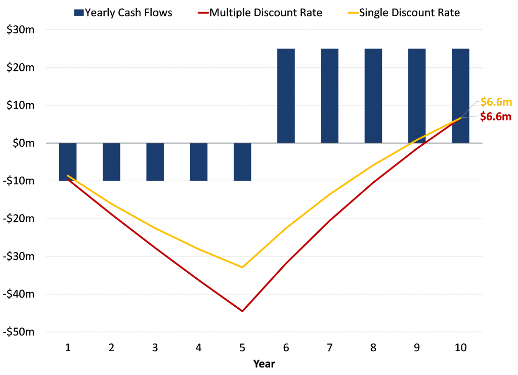
Consider the same hypothetical scenario presented in the previous section, with a firm with projected cash flows over a ten-year period, consisting of negative $10 million per year in years one through five, and positive $25 million per year in years six through ten.
As shown in the previous section, the present value of this cash flow stream under a multiple discount rates approach, where the first five years are discounted at a risk-free rate of 4%, and the second five years are discounted at a WACC of 12%, is approximately $6.6 million.
In practical applications, valuation analysts may apply a company’s WACC as a single discount rate across all projected cash flows, implicitly assuming a uniform level of risk throughout the forecast period. In the present example, this translates into applying a 12% discount rate to both the initial five years of negative cash flows and the subsequent five years of positive cash flows. This treatment assumes that all cash flows—regardless of their underlying risk characteristics—should be discounted at the same rate:

The resulting valuation outcome differs substantially from that of the multiple discount rates approach, producing a materially higher present value by a factor of nearly 2.3,[24] despite identical cash flow projections.
Figure 1 below shows the year-by-year comparison of the two methods. The main difference between them is that the multiple discount rates method applies a smaller discount to early losses, whereas the single discount rate applies a much higher rate of 12% to those same negative cash flows—resulting in greater net negative cash flows (in absolute terms) for the former during the early years.
Figure 1: DCF with Single and Multiple Discount Rates Resulting in Different Valuation Outcomes

This highlights the extent to which a methodological choice can influence valuation results. In litigation, such as matters involving damages, shareholder disputes, or bankruptcy proceedings, the choice of discount rates may materially affect outcomes related to liability, compensation, or settlement terms. The example illustrates that even when cash flow projections are held constant, the decision to apply a single or multiple discount rates framework may have outsized effects on the final valuation.
Example 2
In this second scenario, we revisit the same projected cash flows but ask a different question: Is there a single discount rate that produces the same present value as the multiple discount rates model? The answer is yes. By adjusting the discount rate applied uniformly across all ten years, one can identify a rate—approximately 15.8%—that equates the present value of the cash flows to the $6.6 million obtained under the multiple rate approach.

Figure 2 below shows a comparison of the two methods. Although discounting with a single rate of 15.8% results in smaller net negative cash flows in absolute terms during the early loss-making years, the multiple discount rates approach catches up in the later period of positive earnings, as it applies a lower rate of 12% to those cash flows—ultimately resulting in equivalent net cash flows.
Figure 2: DCF with Single and Multiple Discount Rates Resulting in Identical Valuation Outcomes
While this may appear to reconcile the two methodologies in terms of numerical outcome, it raises a conceptual challenge: In this example, the 15.8% rate is neither the firm’s hypothetical cost of capital of 12% nor the risk-free rate of 4%. In fact, it lies outside the range defined by those two benchmarks. It may not reflect any identifiable investment alternative, capital market benchmark, or macroeconomic condition. In other words, while mathematically convenient, the adjusted discount rate here lacks a clear theoretical or empirical foundation, which may weaken its credibility in expert analysis or legal proceedings.
This example reinforces that numerical equivalence does not necessarily guarantee conceptual soundness. In practice, the selection of discount rates, whether single or multiple, should be supported by economic rationale, consistency with market expectations, and alignment with the risks underlying the projected cash flows.
Conclusion
Valuation plays a critical role in many litigation settings, where financial conclusions can influence outcomes related to liability, damages, and settlement terms. DCF is one of the more frequently applied methodologies in these contexts of enterprise valuation, due to its flexibility and grounding in forward-looking projections. Within this framework, the decision to apply a single or multiple discount rates can have a meaningful impact on the resulting valuation.
As demonstrated in the examples, both approaches can produce significantly different outcomes, even when based on the same projected cash flows. While it is sometimes possible to align their numerical results, doing so may require selecting a discount rate that lacks a clear theoretical or empirical reference point. This underscores the importance of articulating the rationale behind discount rate assumptions and ensuring consistency with the underlying risk characteristics of the cash flows.
Ultimately, the appropriate methodology will depend on the specific facts of the case, the nature of the business or asset being valued, and the analytical goals of the valuation exercise. Maintaining transparency in modeling decisions and grounding assumptions in sound economic reasoning are essential across all approaches.
While the discount rate is a critical input, and this article specifically focuses on assumptions related to discount rate selection, other factors also significantly influence the DCF outcome. These include, for example, the length of the projected cash flow period, the size and timing of expected cash flows, the timing of discounting, the assumptions used for terminal value, the growth rates applied during the forecast period (which reflect expectations about how the business or asset will grow over time), and the overall risk profile of the asset or business being evaluated. ↑
U.S. courts have recognized this distinction and adopted multiple-rate approaches where appropriate to reflect phase-specific risk dynamics. See, e.g., S’holder Representative Servs. LLC v. Alexion Pharms., Inc., 341 A.3d 513 (Del. Ch. 2025). ↑
See Richard A. Brealey, Stewart C. Myers & Franklin Allen, Principles of Corporate Finance, 20–45 (Ch. 2: How to Calculate Present Values) (13th ed., McGraw-Hill Education, 2020); Jonathan Berk & Peter DeMarzo, Corporate Finance 246–272 (Ch. 7: Investment Decision Rules) (5th ed., Pearson 2020). ↑
See, e.g., Northwest Inv. Corp. v. Wallace, 741 N.W.2d 782 (Iowa 2007). ↑
See, e.g., Su v. Bensen, No. 19-3178, 2024 U.S. Dist. LEXIS 145404 (D. Ariz. Aug. 15, 2024). ↑
See, e.g., BP Amoco v. Flint Hills Res., No. 05 C 5661, 2009 U.S. Dist. LEXIS 131272 (N.D. Ill. June 4, 2009). ↑
See, e.g., Dietz v. Jacobs, No. 12-1628, 2014 U.S. Dist. LEXIS 37144 (D. Minn. Mar. 21, 2014). ↑
In re Appraisal of Dell Inc. No. 9322-VCL, 2016 Del. Ch. LEXIS 81 (Del. Ch. May 31, 2016). ↑
Andaloro v. PFPC Worldwide, Nos. 20336, 20289, 2005 Del. Ch. LEXIS 125 (Del Ch. Aug. 19, 2005). ↑
This approach is generally more appropriate when a firm undertakes a project consistent with its core operations. For projects that fall outside the firm’s typical business (for example, a utility company investing in a tech startup), the risk profile may differ significantly. In such cases, one may prefer to use a discount rate different from the firm’s overall WACC. ↑
All discounting examples presented in this article assume that cash flows are realized at the end of each year (e.g., t = 1 for year 1, t = 2 for year 2, and so on) and are discounted back to the beginning of the hypothetical study period (i.e., t = 0). ↑
Note that these studies highlight ongoing discussion around the limitations of single-rate DCF models and the potential for alternative methods, such as multi-rate discounting, to address evolving or segmented risk structures within an investment or project. Whether and how these ideas are implemented in practice varies, and their relevance depends on the specific assumptions and characteristics of the valuation at hand. ↑
Geltner and Mei (1995) and Tiwari (1994) show that shifts in interest rates, inflation, and market risk premiums can cause required returns to fluctuate, making the assumption of a constant discount rate unrealistic. Investors, therefore, form expectations at t = 0 not only about future cash flows but also about how discount rates may change as market conditions evolve. See Kashi Nath Tiwari, Single Versus Multiple Discount Rates in Investment Theory, 7 J. Financial & Strategic Decisions 19–42 (1994); David Geltner & Jianping Mei, The Present Value Model with Time-Varying Discount Rates: Implications for Commercial Property Valuation and Investment Decisions, 11 J. Real Estate Fin. & Econ. 119–135 (1995). Empirical evidence further indicates that valuation models incorporating time-varying discount rates better explain observed market values than those assuming a single, constant rate. See Sujata Behera, Does the EVA Valuation Model Explain the Market Value of Equity Better Under Changing Required Return Than Constant Required Return?, 6 Fin. Innovation 9 (2020). ↑
See Vicente Alcaraz, Should Practitioners (Continue to) Use a Single Discount Rate in Large-Scale Project Valuation?, 20 J. Structured Fin. 93 (2014); Ken Fuller et al., The Problem of Discount Rate in Infrastructure Projects: Exploring the Idea of Financial Twins (Feb. 6, 2023) (unpublished manuscript) (SSRN); Babak Jafarizadeh & Reidar B. Bratvold, Project Economics in the Big-Bets Industry: The Integrated Valuation in Practice, 197 J. Petroleum Sci. & Eng’g 108095 (2021). ↑
See Brealey, Myers & Allen, Principles of Corporate Finance 590–613 (Ch. 22: Real Options); Avinash K. Dixit & Robert S. Pindyck, Investment Under Uncertainty (1st ed. Princeton University Press 1994); David Espinoza et al., DNPV: A Valuation Methodology for Infrastructure and Capital Investments Consistent with Prospect Theory, 38 Constr. Mgmt. & Econ. 259–274 (2020). ↑
See, e.g., Brealey, Myers & Allen, Principles of Corporate Finance 228–256 (Ch. 9: Risk and the Cost of Capital), which lists the risk of a dry hole in oil exploration as an example of “bad outcome” that appears to reflect diversifiable risks that would not affect the expected rate of return demanded by investors. ↑
See Brealey, Myers & Allen, Principles of Corporate Finance Ch. 9, which lists the risk of unacceptable side effects of a new drug as an example of “bad outcome” that appears to reflect diversifiable risks that would not affect the expected rate of return demanded by investors. ↑
See Brealey, Myers & Allen, Principles of Corporate Finance 260 (“Diversifiable risks do not increase the cost of capital. They do affect expected cash flows, however.”); Berk & DeMarzo, Corporate Finance 421 (“Firms sometimes try to adjust for this risk by assigning a higher cost of capital to new projects. Such adjustments are generally incorrect, as this execution risk is typically firm-specific risk, which is diversifiable. . . . Of course, this does not mean that we should ignore execution risk. We should capture this risk in the expected cash flows generated by the project.”). ↑
These examples are not intended to imply that any particular methodology is preferred or should be used in any specific industry. Rather, they illustrate scenarios in which varying risk exposures over time have led researchers and practitioners to explore valuation methods that account for such differences. ↑
S’holder Representative Servs. LLC v. Alexion Pharms., Inc., 341 A.3d 513 (Del. Ch. 2025). ↑
See S’holder Representative Servs. LLC v. Alexion Pharms., Inc., 341 A.3d at 547 (“But the risks underlying the metrics in Milestones 2 through 7 are ‘diversifiable.’ A diversifiable risk is one ‘that is peculiar to an individual company.’ Such risks can be ‘diversified away’ through a broad investment portfolio ‘due to the law of large numbers.’ . . . For Milestones 2 through 7, the discount rate is the risk-free rate plus a credit risk premium.” (citations omitted)). ↑
See S’holder Representative Servs. LLC v. Alexion Pharms., Inc., 341 A.3d at 548 (“Milestone 8 is different because the risk associated with its underlying metric is ‘nondiversifiable.’ As the name suggests, nondiversifiable (or ‘systemic’) risk, ‘cannot be fully removed through diversification’ because it is ‘correlated with the market.” . . . Milestone 8’s net sales metric carries nondiversifiable risk. So the milestone’s discount rate must therefore include a risk premium.” (citations omitted)). ↑
The purpose of this example is to demonstrate how the application of multiple discount rates may affect valuation outcomes under certain assumptions. It does not imply that this approach is preferable, superior, or recommended in any given case. The appropriateness of any methodology depends on factors such as the specific context, assumptions, and purpose of the valuation. ↑
$15.1M / $6.6M ≈ 2.3. ↑
